
MAKING THE PROFILES
First of all you are expected to load a FITS file ("FILE"-"LOAD"). Moving the cursor accross the image you can see a current profile in the first profile window. The profile is corresponding to the position and size of rectangle area. The width of rectangle can be changed by pressing left and right mouse button. The height is controled by the box slider. Actual width and position of the rectangle in the image is shown under the image window. Note: Cursor should always be in the left bottom corner of rectangle but equalization of cursor and rectangle can be slow sometimes.
By pressing the middle button you copy the profile from the first profile window to the second one. The profile in the second window is filtered according to the value of filter slider. Filtering uses the function SMOOTH.
By "REGION" button you can choose if the X axis should be re-counted to the wavelength. If you click on "SLIT JAW" (default), there will be no modification of X axis. Choosing the second possibility, you are supposed to fill in the coefficients of dispersion curve. You can extract them from "*.cfs" file (result of CALIB) or "coef.dat". If you don't know this coefficients you can choose the third possibility. Then you are expected to fill in the position and wavelength of spectral lines (two at least).
By "CALIBRATION" button you can choose if the Y axis should be re-counted or not. If you choose "NO CALIBRATION" (default), there will be no modification of Y axis. Choosing "CALIBRATION", Y axis will be re-counted according to the coefficients a, b, c (the result of CALIB procedure). Note: Calibrated profile can be seen during saving. The result intensities are in % of solar center continuum.
XLOOK offers a possibility of counting a ratio of two integral intensities. The first integral corresponds to the profile in the second profile window and its value is shown below. The ratio of integrals will apear next to the value of the first integral just after clicking on "INTEGRAL"-"MARK QUIET REGION" and marking the region for second profile. If you have filled in the coefficients of calibration, the integrals will be counted from calibrated profiles.
The "SUBTRACT" button gives us the possibility of subtracting of two profiles. In XLOOK
there are two ways how you can get the subtract.
First way: First profile corresponds to the profile in the second profile window. The
second profile (which is subtracted from the first one) you extract after clicking on
"SUBTRACT"-"MARK QUIET PROFILE" and marking the region. Then you will see the result
and you have possibility to save it as a "*.fts". The starting and ending positions are the same
for both profiles and correspond to the first one. Resulting profile is calibrated if you filled
in the coefficients of calibration.
Second way: The second way how to get subtract of two profiles is to click on
"SUBTRACT"-"POSITIONS FOR SUBTRACT" and fill the positions:
The profile depicted in the second profile window can be saved by clicking on "FILE"-"WRITE". Immediately you will see the same profile as it's going to be saved (with re-counted X and Y axis). Information about the saved profile (the region the profile was taken from, the coefficients of dispersion curve, the calibration coefficients, the values of integrals) can be found in the file "tab.dat". The profile is saved as a two row matrix to a FITS file and can be plotted by "plot, file(*,0), file(*,1)".
CORRECTION OF THE COEFFICIENTS OF DISPERSION
The dispersion coefficients of the images taken at the same day shouldn't be much different. Nevertheless these coefficients taken as the result of CALIB aren't exactly the same and that's why XLOOK contains the "LOAD SERIES" section for correction of the coefficients.
After clicking on the "LOAD SERIES" button choose series of images by means of "ADD" and "DELETE" button and choose which region you are going to work with. XLOOK will load the first image. You are supposed to take a profile by clicking middle mouse button and fill in the coefficients of calibration.
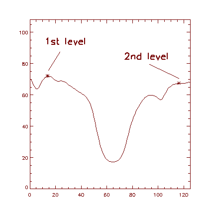
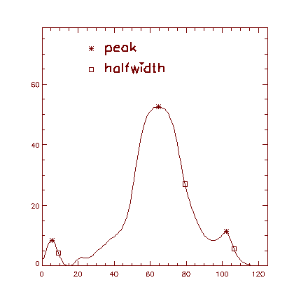
After clicking on the "SERIES-GAUSS" button you will see the selected profile and you are expected to fill in x-position of two continuum levels acording the profile will be rotated to. Then fill in the parameters of spectral lines (you must describe first two lines at least) and XLOOK will interleave the profile with Gaussian curves.
Example of filling contunuum levels and parameters of lines:


Applying this procedure to the next images from the series the XLOOK will plot the dispersion curve, count the coefficients of dispersion for all the images and save them into the file "coef.dat". Note: Working with the next images you are supposed to choose a profile at the same x-position and of the same width as the first one, otherwise the results will be wrong.
Author of the procedure: Eva Havlickova (ehavlickova@centrum.cz)