'corr.jpg'
'hist.jpg'

This program was created for correlating chosen regions in the series of fts images. Here I give the instructions and some results. Data I worked with can be found in 'e:\medon' directory (13th of October 2001 series). The middle picture of the series is used in the program as an instrumental image.
When we start the program first time, we follow the points 1, 2 and 3.
1. 'FILE' - 'LOAD'We load the directory containing the series of images. The following selection will appear:
'Whole image' section is connected with calculations relating to the whole image. 'Chosen regions' section is connected with calculations relating to chosen regions. The images in working directory are taken in alphabetical precedence.
ℑ
2. 'OPTIONS' - 'WHOLE IMAGE' - 'COUNT INTEGRALS'Now we create a grid of regions we are going to work with. As an example, I give my values for the series mentioned above:
Start point is the left bottom corner of the grid and step is the size of square region of the grid in pixels. We can get these parameters by means of 'sit.pro' procedure.
In this section the program counts the integral for each region of the grid for each image. We get a row of integrals for each region. As a matter of fact, the integral is total brightness of the region and it is counted by 'int_tabulated' IDL function. The brightness of images is changing during the series, so we substract the average value of the integrals in given image in addition. The results are saved to 'variable.dat', 'average.dat' and 'region.dat' files.
ℑ
3. 'OPTIONS' - 'WHOLE IMAGE' - 'COUNT CORRELATION COEFFICIENTS'The correlation coefficients for each pair of regions are counted here (we correlate the brightness of the regions, it means two rows of integrals). During the calculations we can see which regions have been already counted. The results are saved to 'koeficienty.dat' file.
ℑ
The computations in section number 2 and 3 are time consuming. In my case, the counting of integrals lasted 2 hours and the counting of the correlation coefficients lasted about 1 hour. The next time we start the program for the same series, we can omit these sections. The program tests the existence of files with the results and it takes data from them.
If we have already counted the integrals and the correlation coefficients, we choose from the following sections:
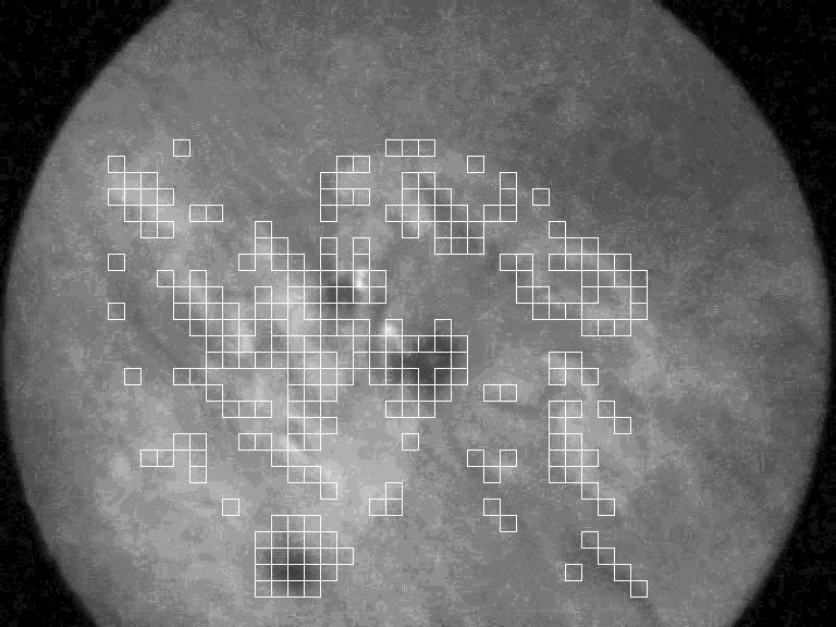
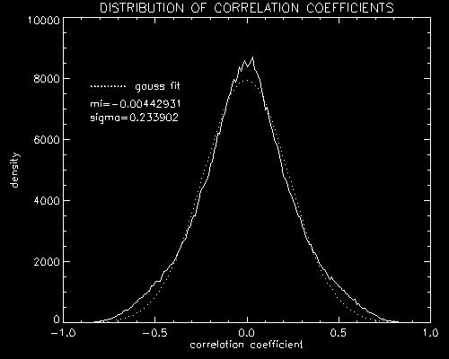
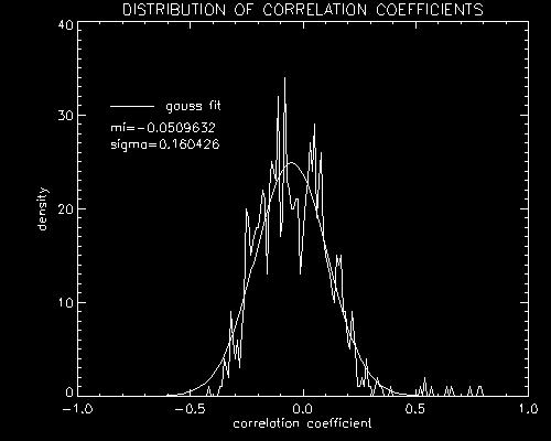
4. 'OPTIONS' - 'WHOLE IMAGE' - 'SHOW REGIONS WITH HIGH CORRELATION'The histogram of all the correlation coefficients and its parameters μ and σ are counted here. In the result image we can see the regions which have high value of the correlation coefficient c (c > μ+3σ or c < μ-3σ) with one other region at least. The results can be saved as 'corr.jpg' and 'hist.jpg' files. We can notice in the following example, that regions with high value of the correlation coefficient correspond to the active regions, the spots and the filaments.
'corr.jpg'
'hist.jpg'
ℑ
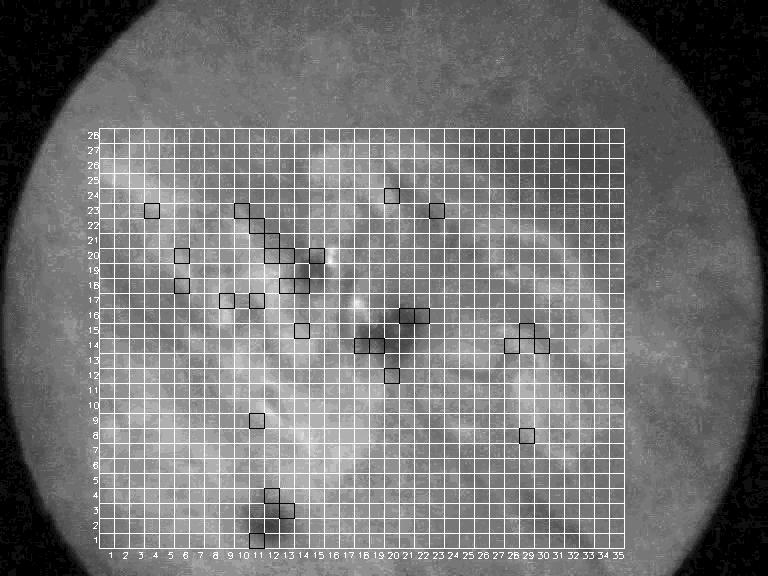
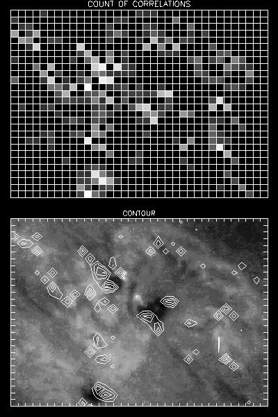
5. 'OPTIONS' - 'WHOLE IMAGE' - 'SHOW REGIONS WHICH CORRELATE WITH TOO MANY REGIONS'In this section, the program looks for the regions, which correlate with too many other regions. We fill 'n' parameter. The program will show the regions, that correlate with more than n regions. Their coordinates can be used in the section number 9. In addition, the program will show the count of the regions which correlate with the corresponding region (the brighter region means the bigger count) and its contour. We can save the results as 'reg.jpg' and 'count.jpg' files. 55 was used as 'n' in the following example.
ℑ
6. 'OPTIONS' - 'CHOSEN REGIONS' - 'AUTO CORRELATION'The autocorrelation of brightness for a chosen region and its Fast Fourier Transform is counted in this section. We fill in the coordinates of the region according to the shown image. We can save the graph as 'auto.jpg' file. The following example was created for the region with coordinates 10,10.
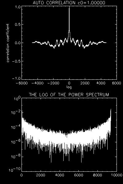
ℑ
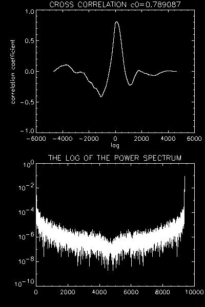
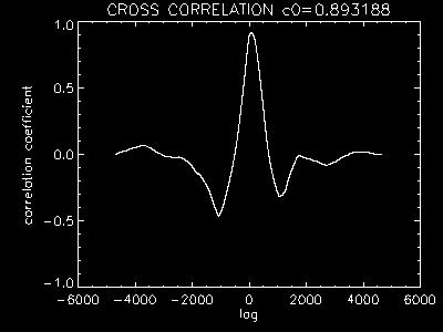
7. 'OPTIONS' - 'CHOSEN REGIONS' - 'CROSS CORRELATION'The correlation of brightness of two chosen regions and its Fast Fourier Transform is counted here. We can save the graph as 'cross.jpg' file. The following example was created for the regions with coordinates 18,17 and 16,20.
ℑ
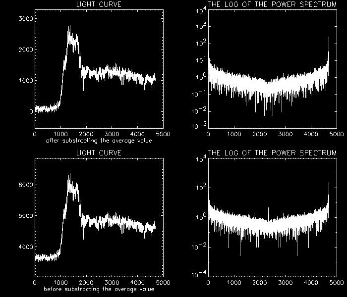
8. 'OPTIONS' - 'CHOSEN REGIONS' - 'LIGHT CURVE'In this section we can get two light curves of a chosen region (the value of the integral versus the number of the image) and their Fast Fourier Transform. First one is made after substracting the average value of the integrals and the second one is made before this substracting. We can save the graphs as 'light.jpg' file. The following example was created for the region with coordinates 16,20.
ℑ
9. 'OPTIONS' - 'CHOSEN REGIONS' - 'DISTRIBUTION'In this section the program looks for the regions which our chosen region correlates with. You fill in the coordinates of the region and choose which histogram you are going to count. In the result image, we can see the regions which our chosen region correlates with (c > μ+3σ or c < μ-3σ). These have white color and the chosen region have black color. The results can be saved as 'corr1.jpg' a 'hist1.jpg' files.
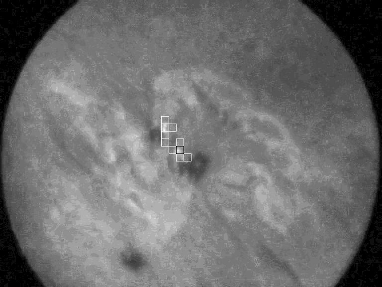
ℑ
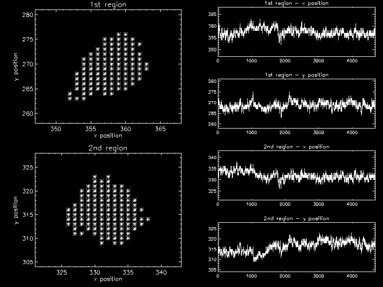
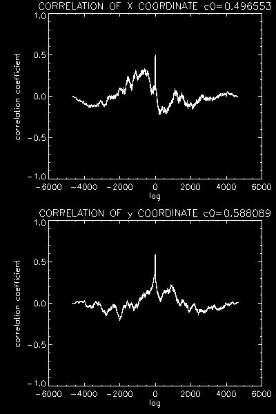
10. 'OPTIONS' - 'CORRECTION'The correlation of brightness of two chosen regions containing the bright points is counted here. The positions of the regions are not fixed, but they move according to the motion of the bright points.
We fill in the coordinates of the regions and choose the way of the correction ('center of brightness' or 'the brightest points'). The regions will then copy the motion of the center of brightness or the brightest point (the center of brightness or the brightest point will always be in the center of the regions).
If the bright points will appear during the series and they are not contained in the first images, the regions can move out of the space where the bright points will appear. In this case we fill in the 'start image' box. It's the number of the image we want to make the correction from. The position of the regions will be fixed in the images with lower number. If we want to make the correction from the beginning, we leave this box empty. We can see the actual position of the regions in the animation running during the calculations.
The results of this section:
These results are automatically saved to 'correct1.jpg', 'correct2.jpg' and 'correct3.jpg' files. The following examples were created for the regions with coordinates 18,17 and 16,20.
Notes:
Author of the procedure: Eva Havlíčková (ehavlickova@centrum.cz)